We will now show an example of value iteration proceeding on a problem for a horizon length of 3. This example will provide some of the useful insights, making the connection between the figures and the concepts that are needed to explain the general problem. For this problem, we assume the POMDP has two states, two actions and three observations.
We start with the first horizon. The value function here will represent the best we can hope to do (in terms of value) if we are limited to taking a single action. This is the simplest case; normally (for horizon length h) we need to trade off the immediate rewards and the future rewards. However, when you have a horizon of 1, there is no future and the value function becomes nothing but the immediate rewards.
Since we have two states and two actions, our POMDP model will include four separate immediate reward values: there is one value for each combination of action and state. These values are defined over the discrete state space of the POMDP, but it becomes easy to get the value of doing a particular action in a particular belief state. To do this we simply use the probabilities in the belief state to weight the value of each state.
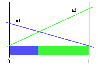
As an example: let action a1 have a value of 0 in state s1 and 1 in state s2 and let action a2 have a value of 1.5 in state s1 and 0 in state s2. If our belief state is [ 0.75 0.25 ] then the value of doing action a1 in this belief state is 0.75 x 0 + 0.25 x 1 = 0.25. Similarly, action a2 has value 0.75 x 1.5 + 0.25 x 0 = 1.125. We can display these values over belief space with the figure below. This is, in fact, the horizon 1 value function. (Note that we have not violated the "no formula" promise: what preceded were not formulas, they were just calculations.)
|
Horizon 1 value function
The immediate rewards for each action actually specifies a linear function over belief space. Since we are interested in choosing the best action, we would choose whichever action gave us the highest value, which depends on the particular belief state. So we actually have a PWLC value function for the horizon 1 value function simply by considering the immediate rewards that come directly from the model. In the figure above, we also show the partition of belief space that this value function imposes. Here is where the colors will start to have some meaning. The blue region is all the belief states where action a1 is the best strategy to use, and the green region is the belief states where action a2 is the best strategy.
With the horizon 1 value function we are now ready to construct the horizon 2 value function. This part of the tutorial is the most crucial for understanding POMDP solutions procedures. Once you understand how we will build the horizon 2 value function, you should have the necessary intuition behind POMDP value functions to understand the various algorithms.
Our goal in building this new value function is to find the best action (or highest value) we can achieve using only two actions (i.e., the horizon is 2) for every belief state. To show how to construct this new value function, we break the problem down into a series of steps.
- We will first show how to compute the value of a single belief state for a given action and observation.
- Then we show how to compute the value for every belief state for a given action and observation, in a finite amount of time.
- Then we will show how to compute the value of a belief state given only an action.
- Finally, we will show how to compute the actual value for a belief state.
Computing a Belief State Value from an Action and Observation
We start with the problem: given a particular belief state, b what is the value of doing action a1, if after the action we received observation z1? In other words we want to find the best value possible for a single belief state when the immediate action and observation are fixed.
The value of a belief state for horizon 2 is simple the value of the immediate action plus the value of the next action. In general, we would like to find the best possible value which would include considering all possible sequences of two actions. However, since in our restricted problem our immediate action is fixed, the immediate value is fully determined. We can use the immediate rewards for action a1 to find the value of b just like we did in constructing the horizon 1 value function. Recall that the horizon 1 value function is nothing but the immediate reward function.
The only question is what is best achievable value for the belief state that results from our initial belief state b when we perform action a1 and observe z1. This isn't really much of a problem at all, since we know our initial belief state, the action and the resulting observation. This is all that is required to transform b into the unique resulting next belief state, which we will call b'. This new belief state will be the belief state we are in when we have one more action to perform; our horizon length is 2, but we just did one of the 2 possible actions. We know what the best values are for every belief state when there is a single action left to perform; this is exactly what our horizon 1 value function tells us.
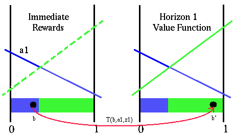
The figure below shows this process. On the left is the immediate reward function and on the right is the horizon 1 value function. (Recall that for horizon length 1, the immediate rewards are the same as the value function.) The immediate rewards for action a2 are shown with a dashed line, since they are not of immediate interest when considering the fixed action a1.
|
Value of a fixed action and observation
Here we will define T as the function that transforms the belief state for a given belief state, action and observation (the formulas are hiding in here). Note that from looking at where b' is, we can immediately determine what the best action we should do after we do the action a1. The belief state b' lies in the green region, which means that if we have a horizon length of 2 and are forced to take action a1 first, then the best thing we could do afterwards is action a2.
Recall that what we are concerned with at this point is finding the value of the belief state b with the fixed action and observation. We have everything we need to calculate this value; we know what the immediate reward we will get is and we know the best value for the transformed belief state b'. Simply summing these two values gives us the value of belief state b given that we take action a1 and observe z1. As a side effect we also know what is the best next action to take.
Computing All Belief State Values for an Action and Observation
Suppose we want to find the value for another belief state, given the same action and observation. We simply repeat this process, which means all that we really need to do is transform the belief state and use the horizon 1 value function to find what value it has (the immediate rewards are easy to get). Now suppose we want to find the value for all the belief points given this fixed action and observation. This seems a little harder, since there are way to many points we have to do this for. Fear not, this can actually be done fairly easily.
As we compute the horizon 2 value function for a given initial belief state, action and observation, we would transform the belief state to anew point in belief space and use the horizon 1 value function to simply lookup the value of this transformed space. Suppose we ignore worry about factoring in the immediate rewards before transforming the belief state. Imagine we plotted this function: for every belief state, transform it (using a particular action and observation) and then lookup the horizon 1 value of the new belief. This would give you another value function over belief space, which would be the horizon 1 value function, but slightly transformed from the original. The transformation results from having factoring in the belief update calculation.
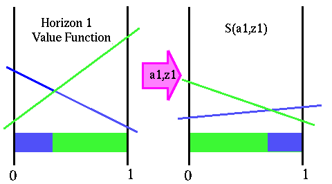
This imaginery algorithm cannot actually be implmented directly since there are uncountably infinite number of belief states we would need to do this for. However, it turns out that we can directly construct a function over the entire belief space from the horizon 1 value function that has the belief transformation built in. This gives us a function which directly tells us the value of each belief state after the action a1 is taken and observation z1 is seen without having to actually worry about transforming the belief state. The figure below show this transformation.
|
Transformed value function
We will use S() to represent the transformed value function, for a particular action and observation. The very nice part of this is that the transformed value function is also PWLC and the nicer part is that it always is this way. (Sorry, the proof requires formulas and we can't do those here.) Now if we want to find the value of a belief state for the fixed action and observation we can just add the immediate rewards for the belief state and add the value we directly get from the transformed function S(a1,z1). In fact we could just add these two functions (immediate rewards and the transformed horizon 1 value function) together to get a single function for the value of all belief points, given action a1 and observation z1. (Note: this is a slight lie and we will explain why a bit later.)
Computing a Belief State Value for a Single Action
We previously decided to solve the simple problem of finding the value of a belief state, given a fixed action and observation. We have showed this and actually demonstrated how to find the value of all belief states given a fixed action and observation. Next we want to show how to compute the value of a belief state given only the action.
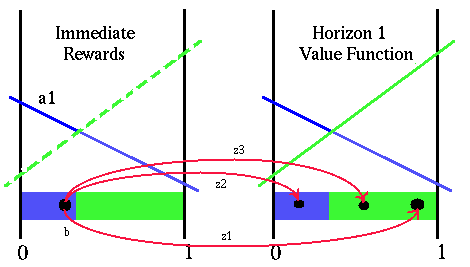
When we were looking at individual points, getting their immediate reward value, transforming them and getting the resulting belief states value, we where computing the conditional value. This is the value if we see observation z1. However, because the observations are probabilistic, we are not guaranteed to see z1. In this example, there are three possible observations and each one can lead to a separate resulting belief state. This figure below, shows the full situation when we fix our first action to be a1.
|
Transformed value function
Even though we know the action with certainty, the observation we get is not known in advance. To get the true value of the belief point b we need to account for all the possible observations we could get. The assumption that we knew the resulting observation was a convenience to explain how the process works, but to build a value function for horizon 2 we need to be able to compute the value of the belief states without prior knowledge of what the outcome will be. All of this is really not that difficult though. For a given belief state, each observation has a certain probability associated with it. If we know the value of the resulting belief state given the observation, to get the value of the belief state without knowing the observation is just a matter of weighting each resulting value by the probability that we will actually get that observation.
This might still be a bit cloudy, so let us do an example. Suppose that we compute the values of the resulting belief states for belief state b, action a1 and all three observations and find that the values for each resulting belief state are: z1:0.8, z2:0.7, z3:1.2. These are the values we were initially calculating when we were doing things one belief point at a time. Now we also can compute the probability of getting each of the three observations for the given belief state and action and find them to be: z1:0.6, z2:0.25, z3:0.15. Then the horizon 2 value of the belief state b when we fix the action at a1 is 0.6x0.8 + 0.25x0.7 + 0.15x1.2 = 0.835 plus the immediate reward of doing action a1 in b.
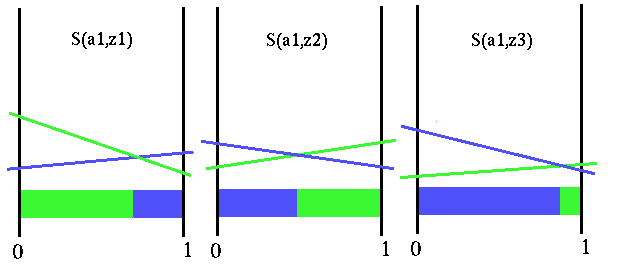
In fact, the transformed value function S(a1,z1) we showed before actually factors in the probabilities of the observation. So in reality, the S() function is not quite what we claimed; we claimed that it was the next belief state value of each belief state for the fixed action and given the observation. It reality, the S() function already has the probability of the observation built into it.
Let's look at the situation we currently have with the figure below.
|
Transformed value function for all observations
This figure shows the transformation of the horizon 1 value function for the action a1 and all three observations. Notice that the value function is transformed differently for all three observations and that each of these transformed functions partitions the belief space differently. How the value function is transformed depends on the specific model parameters. What all this implies is that the best next action to perform depends not only upon the initial belief state, but also upon exactly which observation we get.
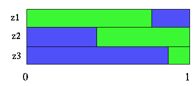
So what is the horizon 2 value of a belief state, given a particular action a1? Well, it depends not only on the value of doing action a1 but also upon what action we do next (where the horizon length will be 1). However, what we do next will depend upon what observation we get. For a given belief state and observation, we can look at the S() function partition to decide what the best action next action to do is. This is best seen with a figure.
|
Partitions for all observations
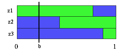
This figure is just the S() partitions from the previous figure displayed adjacent to each other. The blue regions are the belief states where action a1 is the best next action, and the green regions are where a2 would be best. Now let's focus on the problem of finding the best value of a belief state b given that the first action is fixed to be a1. We will use the point shown in the figure below.
|
Belief point in transformed value function partitions
What we see from this figure is that if we start at the belief point b, do action a1, then the next action to do would be a1 if we observer either z2 or z3 and action a2 if we observe z1. The figure above allows us to easily see what the best strategies are after doing action a1. If you recall that each of the partition regions actually corresponds to a line in the S() function, we can easily get the value of the belief point b. We take the immediate reward we get from doing action a1 and add the value of the functions S(a1,z1),S(a1,z3), S(a1,z3) at belief point b.
Computing the Final Belief State Value
In fact, if we fix the action to be a1 and the future strategy to be the same as it is at point b (namely: z1:a2, z2:a1, z3:a1) we can find the value of every single belief point for that particular strategy. To do this we simply sum all of the appropriate line segments. We use the line segment for the immediate rewards of the a1 action and the line segments from the S() functions for each observation's future strategy. This gives us a single linear segment (since adding lines gives you lines) over all belief space representing the value of adopting the strategy of doing a1 and the future strategy of (z1:a2, z2:a1, z3:a1). The notation for the future strategies just indicates an action for each observation we can get.
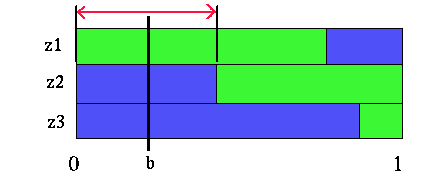
We derived this particular future strategy from the belief point b and it is the best future strategy for that belief point. However, just because we can compute the value of this future strategy for each belief point, doesn't mean it is the best strategy for all belief points. So which belief points is this the best future strategy? This is actually easy to see from the partition diagram.
|
Belief point in transformed value function partitions
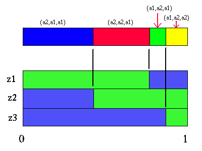
The region indicated with the red arrows shows all the belief points where the future strategy (z1:a2, z2:a1, z3:a1) is best (given that action a1 is taken first). Since there are three observations and two actions, there are a total of 8 possible different future strategies. However, some of those strategies are not the best strategy for any belief points. Given the partitioning figures above, all the useful future strategies are easy to pick out. For our example, there are only 4 useful future strategies. The figure below shows these four strategies and the regions of belief space where each is the best future strategy.
|
Partition for action a1
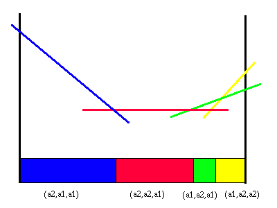
Each one of these regions corresponds to a different line segment in the value function for the action a1 and horizon length 2. Each of these line segments is constructed as we indicated before by adding the immediate reward line segment to the line segments for each future strategy. If we created the line segment for each of the four future strategies from the figure above, we would get a PWLC function that would impose exactly the partition shown above. This value function is shown in this next figure.
|
Value function and partition for action a1
Note that each one of these line segments represents a particular two action strategy. The first action is a1 for all of these segments and the second action depends upon the observation. Thus we have solved our second problem; we now know how to find the value of a belief state for a fixed action. In fact, as before, we have actually shown how to find this value for every belief state.
If there was only the action a1 in our model, then the value function shown in the previous figure would be the horizon 2 value function. However, because there is another action, we must compare the value of the other action with the value of action a1 before we have the true horizon 2 value function, since we are interested in finding the best value for each belief state.
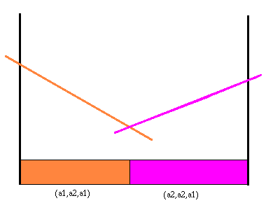
We can repeat the whole process we did for action a1 for the other action. This includes constructing the S() functions for the action a2 and all the observations. From these we can find the value function for that action. Below is the value function and partition for action a2.
|
Value function and partition for action a2
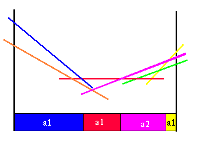
In this case there happens to be only two useful future strategies. We can put the value functions for each action together to see where each action gives the highest value.
|
Combined a1 and a2 value functions
We can see that from this picture that there is only one region where we would prefer to do action a2. Everywhere else, this action is not as good as action a1. We can see that one of the line segments from each of the two action value functions are not needed, since there are no belief points where it will yield a higher value than some other immediate action and future strategy. Here is the more compact horizon 2 value function.
|
Value function for horizon 2
The partition shown below the value function in the figure above shows the best horizon 2 policy, indicating which action should be taken in each belief state. Notice that there are three different regions, two of which are adjacent, where we choose action a1. These regions are distinguished because, although the initial action is the same, the future action strategies will be different.
This whole process took a long time to explain and is not nearly as complicated as it might seem. We will show how to construct the horizon 3 policy from the horizon 2 policy is a slightly accelerated manner. The steps are the same, but we can now eliminate a lot of the discussion and the intermediate steps which we used to aid the explanation.
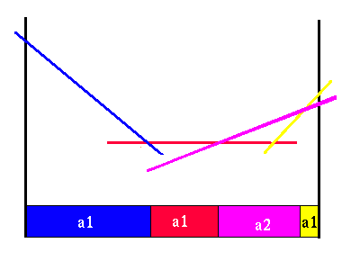
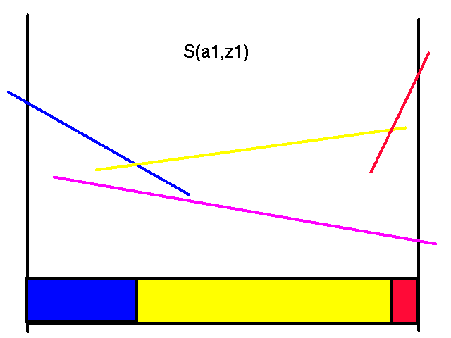
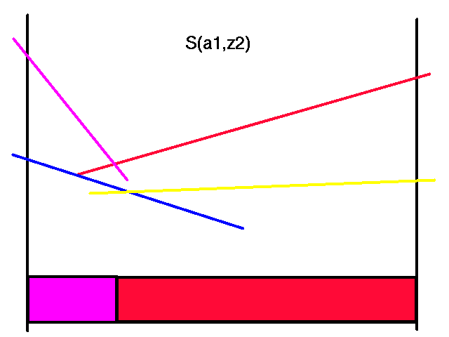
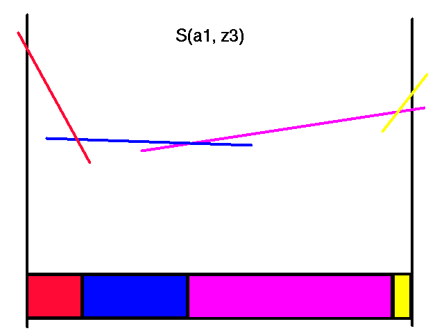
First transform the horizon 2 value function for action a1 and all the observations.
|
|
|
Transformed Horizon 2 Value Functions for Action a1
Note that each of the colors here corresponds to the same colored line in the horizon 2 value function. Also note that not all of the transformed lines become useful in the representation of the maximal values.
When we were constructing the horizon 2 value function, these colors corresponded to the next action to take. The reason the colors corresponded to a single action was that with a horizon length of 2, there was only going to be a single action left to take after taking the first action. However, here and in general, each color represents a complete future strategy, not just one action. For instance, the magenta color corresponds to the line in the horizon 2 value function where we would do the action a2 and adopt its future strategy. The future strategy of the magenta line will depend on the observation we get after doing the a2 action.
Next we find the value function by adding the immediate rewards and the S() functions for each of the useful strategies. The partition that this value function will impose is easy to construct by simply looking at the partitions of the S() functions.
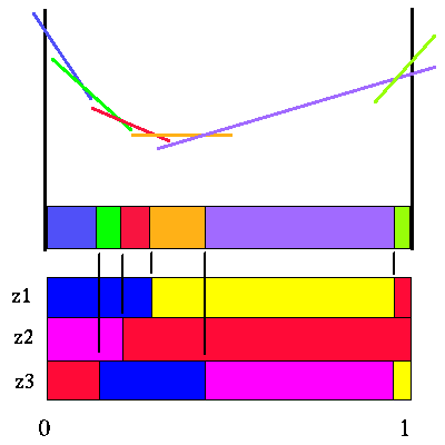
In the figure below, we show the S() partitions for action a1 below and the value function for action a1 with a horizon of 3. The partition this value function imposes is also shown.
|
Value function for action a1 and horizon 3
Note that for this action, there are only 6 useful future strategies, which are represented by the partitions that this value function imposes on the belief space.
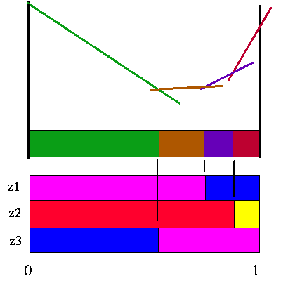
We then construct the value function for the other action, put them together and see which line segments we can get rid of. Here are the S() function partitions, value function and the value functions partition for the action a2.
|
Value function for action a2 and horizon 3
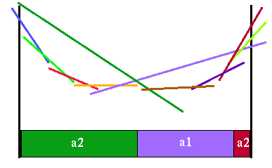
Note that there are only 4 useful future strategies for the action a2. Here are the a1 and a2 value functions superimposed upon each other.
|
Value functions for both actions a2 and horizon 3
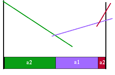
Note how many line segments get completely dominated by line segments from the other action's value function. The final horizon 3 value function looks like this:
|
Value function for horizon 3
Note that this value function is much simpler than the individual action value functions. It is even simpler than the horizon 2 value function. Whether the resulting function is simpler or more complex depends upon the particular problem. These examples are meant to show how you can get either one; i.e., the value functions do not have to get more complex as we iterate through the horizons.
This concludes our example. The concepts and procedures can be applied over and over to any horizon length. This is the way we do value iteration on the CO-MDP derived from the POMDP.
Continue
 POMDP.org